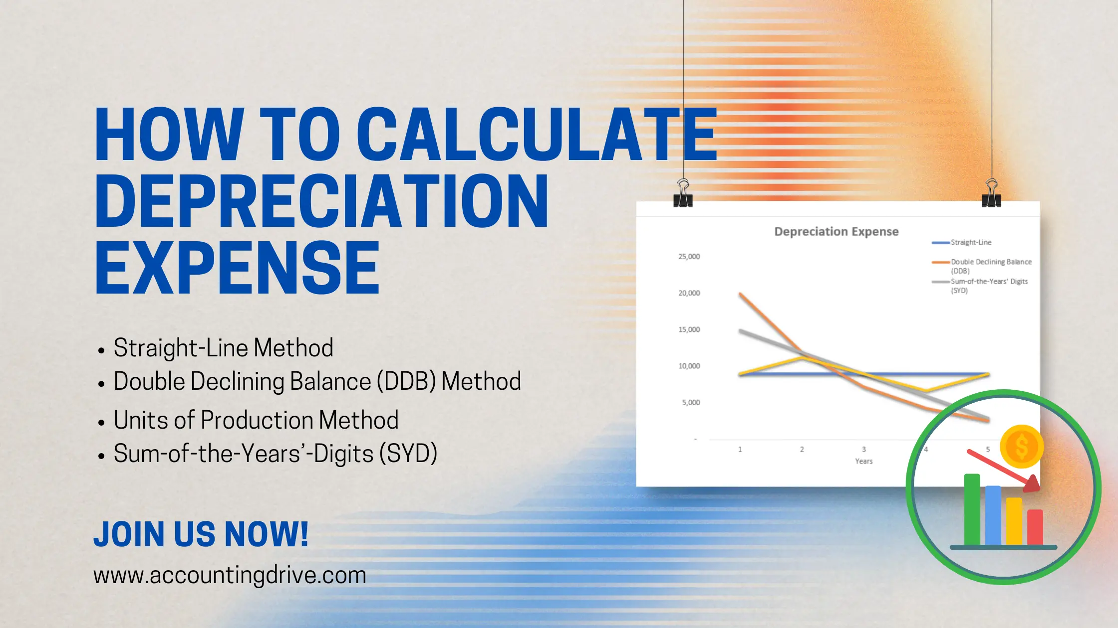
Are you a student trying to understand how to calculate depreciation expense for your accounting exams? It’s a core part of accounting education. And for entrepreneurs, mastering depreciation is essential for smart financial management and asset planning. Depreciation helps allocate the cost of long-term assets over their useful life, impacting everything from financial statements to tax deductions. In this post, we’ll explore the 4 methods of depreciation—Straight-Line, Double Declining Balance, Sum-of-the-Years’ Digits, and Units of Production. With simple formulas, real-world examples, and a detailed comparison, you’ll be able to confidently apply the right depreciation method whether you’re studying for an exam or managing business finances.
What is Depreciation?
In This Article
ToggleDepreciation is the process of allocating the cost of a fixed asset over its useful life. It reflects the asset’s wear and tear, helping businesses track its declining value over time. Depreciation not only affects a company’s financial statements but also has tax implications.
For businesses, calculating depreciation accurately is crucial for managing financials and making informed decisions.
Key Terms
Salvage Value/ Residual Value: The estimated value of an asset at the end of its useful life.
Useful Life: The period during which an asset is expected to be usable.
Book Value: The value of an asset on the balance sheet after deducting accumulated depreciation. Formula: Original cost – Accumulated depreciation
Accumulated Depreciation: The total depreciation expense that has been recorded against an asset since it was acquired.
Depreciable Amount: The portion of the asset’s cost that will be depreciated over time. Formula: Cost of Asset – salvage value.
Cost of Asset: The total amount paid to acquire and prepare an asset for use, including purchase price, installation costs, delivery fees, and other related expenses.
Format for Calculation of the Total Cost of a Fixed Asset
The total cost of a fixed asset includes all expenses incurred to acquire, transport, install, and prepare the asset for use in business operations.
Description | Amount |
Purchase Price | $_____ |
(-) Trade Discount | $_____ |
(-) Cash Discount | $_____ |
Net Purchase Price | $_____ |
(+) Installation Costs | $_____ |
(+) Transportation and Handling Costs | $_____ |
(+) Taxes and Duties | $_____ |
(+) Legal or Licensing Fees | $_____ |
(+) Other Costs (e.g., Training, Site Prep) | $_____ |
Total Cost of the Fixed Asset | $_____ |
Explanation
Purchase Price: The initial amount paid to buy the asset.
Trade Discount: A discount provided by the seller based on the volume or nature of the purchase.
Cash Discount: A discount offered for making an early payment or paying in cash.
Installation Costs: Expenses related to installing the asset, making it ready for operation (e.g., setup fees, labor costs).
Transportation and Handling Costs: Any shipping, delivery, and handling costs to get the asset to your business location.
Taxes and Duties: Any sales tax, import duty, or other related taxes paid at the time of asset purchase.
Methods to Calculate Depreciation Expense
Method | Formula | Description |
Straight-Line Method | (Cost–Salvage Value) ÷ Useful Life | Depreciates evenly over the asset’s useful life. |
Double Declining Balance (DDB) Method | Book Value at Start of Year × Depreciation Rate | Higher depreciation in the early years, decreasing over time. |
Units of Production Method | (Cost–Salvage Value) ÷ Total Expected Output × Units Produced | Depreciation based on usage or output. |
Sum-of-the-Years’-Digits (SYD) | (Remaining Life ÷ Sum of the Years Digits) × (Cost–Salvage Value) | Accelerated depreciation method, higher in early years. |
1. Straight-Line Depreciation Method
The most common and simplest method, Straight-Line Depreciation spreads the cost of an asset evenly over its useful life.
Straight-line Depreciation Formula:
Annual Depreciation Expense = (Cost of the Asset − Salvage Value) ÷ Useful Life
Interpretation: The Straight-Line Method is simple and gives equal depreciation each year. It’s ideal for assets that lose value uniformly.
Key Points:
- Easy to calculate.
- Provides consistent expense each year.
- Best suited for assets that depreciate evenly, like buildings or office furniture.
Interesting Fact: Over 80% of small businesses prefer the straight-line method for its simplicity and straightforward financial planning.
2. Double Declining Balance (DDB) Depreciation Method
This is an accelerated depreciation method that applies a higher depreciation rate in the early years of the asset’s life. The most common variation is the Double Declining Balance method.
Formula:
Depreciation Expense = Book Value at Start of Year × Depreciation Rate
In the case of Double Declining Balance:
Depreciation Rate = 2÷Useful Life
Interpretation: This method depreciates assets faster in the earlier years, reflecting rapid loss in value. It’s often used for tech equipment or vehicles, which lose value quickly.
Key Points:
- Higher expense in the early years, lower in later years.
- Good for assets that lose value faster, like technology or vehicles.
Interesting Fact: Many tech companies favor this method for gadgets and hardware since 40-60% of an asset’s value might diminish in the first few years due to rapid obsolescence.
3. Units of Production Method
This method bases depreciation on actual usage, making it perfect for machinery, vehicles, or equipment whose wear and tear depend on how much they are used.
Formula:
Depreciation Expense = ((Cost – Salvage Value) ÷ Total Expected Output) × Units Produced
Interpretation: Best for assets whose wear and tear depend on usage, such as machinery or production equipment.
Key Points:
- Tied directly to asset usage.
- Most accurate for production-heavy industries like mining or transportation.
Interesting Fact: This method is used by 60% of mining companies to reflect depreciation based on the actual depletion of resources.
4. Sum-of-the-Years’-Digits (SYD) Method
Another accelerated method, SYD allocates depreciation based on the sum of the years of the asset’s useful life. More depreciation occurs in the earlier years.
Formula:
Depreciation Expense = (Cost–Salvage Value) × (Remaining Life ÷ Sum of the Years Digits)
The Sum of the Years’ Digits is calculated as:
For a 5-year life: 1+2+3+4+5=15
Interpretation: SYD is an accelerated depreciation method, providing higher deductions in the earlier years, making it suitable for assets that depreciate quickly.
Key Points:
- Results in a declining expense over time.
- Ideal for assets that wear out quickly in the initial years, like manufacturing equipment.
Interesting Fact: Studies show that 30% of large manufacturers use SYD to account for machinery depreciation, ensuring accurate financial reporting.
Choosing the Best One
Method | Pros | Cons |
Straight-Line | Simple and predictable | Doesn’t account for varying asset usage |
Double Declining Balance (DDB) | Higher expense in early years, tax benefits | Lower expenses in later years |
Sum-of-the-Years’ Digits | Balances early higher costs with later lower | Complex calculation |
Units of Production | Matches expense with actual use | Requires tracking of usage data |
Which is better?
The right method depends on your business needs:
- Straight-Line is ideal if you want a consistent expense every year.
- Double Declining Balance is useful for assets that lose value quickly and when you want tax benefits in the early years.
- Sum-of-the-Years’ Digits offers similar benefits to DDB but slightly less aggressive.
- Units of Production is the best fit for businesses where wear and tear are directly tied to how much the asset is used, like mining or transportation.
By understanding and choosing the right depreciation method, you’ll ensure your financials are in check and your business is prepared for future growth.
Depreciation Methods Example: How to Calculate Depreciation Expense
To make it more simple, let’s compare each method with the same example.
This detailed example and table make it easier to visualize how depreciation expenses change over time with each method.
Scenario:
Assume a business purchases a delivery truck for $50,000. The truck has an estimated useful life of 5 years, and a salvage value of $5,000. The truck is expected to drive 100,000 miles during its lifetime. The business wants to compare how the depreciation expense differs under each of the four methods.
Data:
- Cost of Asset: $50,000
- Salvage Value: $5,000
- Useful Life: 5 years
- Depreciation Rate: 2/5 = 40%
- Total Estimated Units: 100,000 miles
1. Straight-Line Depreciation Example
Straight-line depreciation spreads the depreciation evenly over 5 years.
Formula:
Annual Depreciation Expense = (50,000 – 5000)/ 5 = 9,000
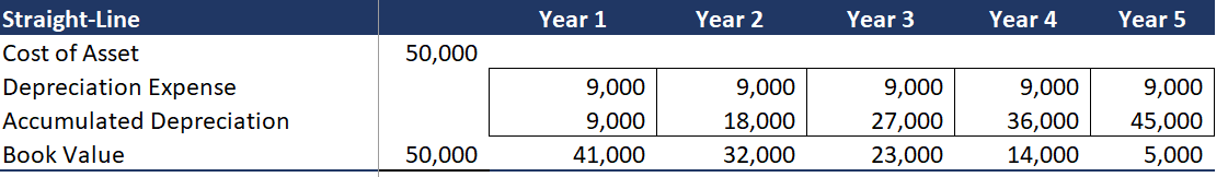
Interpretation:
Each year, the truck will depreciate by $9,000, regardless of how much it is used.
2. Double Declining Balance (DDB) Depreciation Example
DDB front-loads the depreciation, resulting in higher expenses in the earlier years.
Formula:
First, calculate the depreciation rate. Here,
Depreciation Rate = 2 ÷ 5 = 40%
Depreciation Expense = Book Value at the beginning of Year × 40%
For Year 1 | For Year 2 |
50,000 × 40% = 20,000 | (50,000−20,000) × 40% = 12,000 |
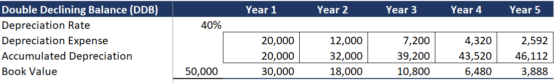
Interpretation:
Depreciation in the first year is $20,000, and it decreases over time as the book value decreases.
3. Sum-of-the-Years' Digits (SYD) Example
This method also results in accelerated depreciation.
Sum of the Years’ Digits: 1+2+3+4+5=15
For Year 1 | For Year 2 |
5 / 15 × (50,000 − 5,000) = 15,000 | 4/15 × (50,000 − 5,000) = 12,000 |
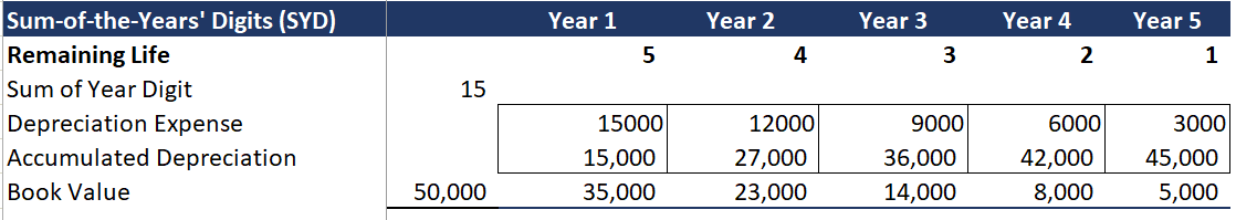
Interpretation:
Depreciation is higher in earlier years, $15,000 in Year 1 and $12,000 in Year 2, but it decreases over time.
4. Units of Production Depreciation Example
This method is based on actual usage, in this case, miles driven.
- Cost of Asset: $50,000
- Salvage Value: $5,000
- Total Estimated Units: 100,000 miles
Formula:
Depreciation Expense = (50,000 − 5,000) × Miles Driven in Year 100,000
If the truck drives 20,000 miles in Year 1:
(50,000 − 5,000) × (20,000/ 100,000) = 9,000
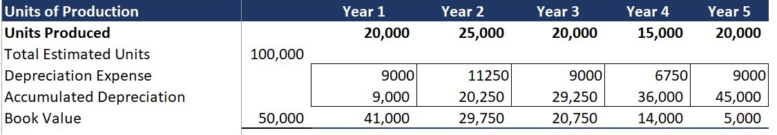
Interpretation:
Depreciation is directly tied to how much the truck is used. For 20,000 miles driven in Year 1, depreciation is $9,000.
Comparison of All Methods
Based on Annual Depreciation Expense
Method | Year 1 Depreciation | Year 2 Depreciation | Total Depreciation After 2 Years | Characteristics |
Straight-Line | $9,000 | $9,000 | $18,000 | Equal annual expense throughout the asset’s useful life. |
Double Declining Balance | $20,000 | $12,000 | $32,000 | Higher depreciation in early years, tax benefits. |
Sum-of-the-Years’ Digits | $15,000 | $12,000 | $27,000 | Accelerated, declining depreciation. |
Units of Production | $9,000 (for 20,000 miles) | $11,250 (25,000 miles) | $20,250 | Depreciation based on usage, is ideal for variable use assets. |
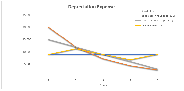
Explanation:
SL (Straight-Line): Consistent depreciation each year ($9,000) until book value reaches salvage value ($5,000).
DDB (Double Declining Balance): The Depreciation Expense is highest in the first year ($20,000) and reduces significantly each year, with the final year’s expense being the smallest ($1,480).
SYD (Sum-of-the-Years’ Digits): Similar to DDB, the Depreciation Expense is higher in the earlier years but follows a smoother decline. Year 1 has $15,000 in expenses, decreasing to $3,000 in the final year.
Units of Production: The Depreciation Expense varies based on usage (miles driven). Year 2 has the highest depreciation ($11,250), reflecting the asset’s higher usage, while years with less usage (Year 4, $6,750) result in lower expenses.
Based on Book Value
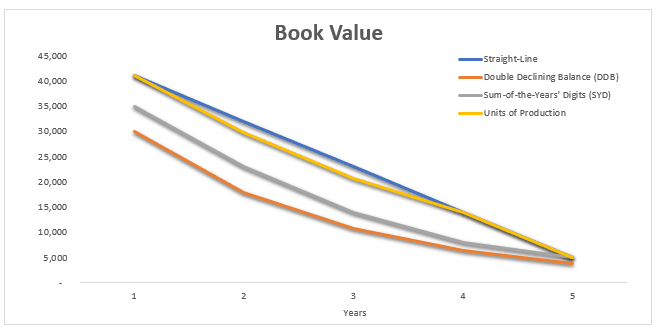
Explanation:
SL (Straight-Line): Book Value decreases by a consistent amount ($9,000) each year. It reaches the salvage value ($5,000) at the end of year 5.
DDB (Double Declining Balance): Here it decreases rapidly in the first few years, losing a larger portion in year 1 ($20,000) and then progressively less each year.
SYD (Sum-of-the-Years’ Digits): It follows a similar pattern to DDB but with a smoother decrease. It drops the most in year 1 ($15,000) and decreases gradually over time.
Units of Production: Here Book Value decreases in direct proportion to the asset’s usage (e.g., miles driven). In year 2, the asset’s book value dropped the most, based on higher usage (11,250).
Conclusion
The key is to match the method with the asset’s actual value consumption. Whether you’re aiming to reflect rapid value loss early on, maintain consistent expenses, or track usage-based wear, understanding these options ensures you optimize your financial strategy and decision-making.
FAQs
Assets such as land do not depreciate, as they don’t lose value over time. Some investments and intangible assets may also not depreciate.
Both the Declining Balance and SYD Methods allocate higher depreciation in the earlier years compared to later ones.
For tax purposes, many businesses opt for Declining Balance or other accelerated methods, as they allow higher depreciation deductions in the early years, reducing taxable income. However, tax rules vary by country, so consult a tax advisor.
Both the Declining Balance and Sum-of-the-Years’-Digits (SYD) methods result in higher depreciation expenses in the early years of an asset’s life compared to the Straight-Line method.
Typically, once a depreciation method is chosen, it’s not easy to change without regulatory or tax authority approval. However, if you find a significant reason, you can consult your accountant or tax advisor about possible options.